#033: Evanescent Acoustic Waves in Tubes
- May 13, 2020
- 8 min read
Updated: Jan 13, 2021
The topic of evanescent fields/waves in any physics can be quite difficult to grasp. It is sometimes explained incorrectly, and looking at books only, it can be difficult to imagine the propagation of the sound field. In this post, I will try to take some of the mystery of the topic, and show some animations and practical aspects for the particular cases of acoustic evanescent waves in tubes.
It is probably best to start with the topic of modes in general(see e.g. this post and this post). Physical structures and enclosures have certain inherent eigenmodes for which they can respond very dramatically to an input. A typical situation is something like a ruler fixed at one end, and flicked with a finger at the other end. The ruler wants to vibrate at a certain (eigen-)frequency and with a certain shape; the eigenfunction, and these two eigen-characteristics together give us the eigenmode.

Now, the modes are not more inherent than they actually depend on the boundary conditions. So if the ruler is fixed midway down its length, its eigenmodes change. If its totally free, the modes change again. Also, there are an infinite number of eigenmodes. So when we see the ruler responds with a particular shape, it is a consequence of the exitation being put at the free end. This excites the first eigenmode very well, so that is what we see. If we excite it differently, we will see a response 'borrowing' from some of the other available modes.
Note: If you see a peak in a response at a certain frequency, it can be a good idea to do an eigen-study, and see if the peak is coming directly from a mode. But just because you find one or more modes around that frequency, does not mean that the peak is the result of these modes. For your particular excitation, the modes may not be excited at all. Conversely, some modes that might be excited, may not be able to create a peak in your particular response; a loudspeaker mode where half of the speaker moves in as the other half moves out is not an efficiently sound source, and so a peak in an on-axis SPL near the same frequency as this mode should not be interpreted as coming from this mode. Not all peaks are modes, and not all modes give peaks!
The prototypical eigenmode 'setup' in acoustics is probably the acoustic modes in a room. You have probably seen this at many instances; a rectangular room has an infinite number of eigenmodes determined by its three dimensions. Below is shown the four lowest for a specific room.

Again it is important to remember that certain boundary conditions have been assumed, typically hard walls, and that no excitation is taken into account in an eigenmode analysis; the response has to be found in a subsequent analysis (see e.g. this post). The scaling of the individual eigenfunctions, i.e. the pressure amplitude that is shown in the figure, is in principle arbitrary (again, see e.g. this post and this post), but inside any simulation software a certain scaling has to take place to actually show something on the screen. You can see in the documentation which method is used in your particular software, but for our discussion don't put any significance on the values of the mode pressures.
Okay, so what about the tubes? Well, all of the above is actually to show now that there is a significant difference between room modes and tube modes. Each room (or 'cavity') mode exists at one particular frequency only. You can excite it more and more with frequencies that are closer and closer to this frequency, but the actual mode has one and only one frequency associated with it. But here is the kicker: Each tube (or 'duct') mode exists at all frequencies! Whereas cavity modes tell you about resonant behavior, tube modes relate to propagation. Without going to much into the mathematical details, the so-called wavenumber for a cavity mode, like the room above, looks something like this:
For each distinct associated eigenfrequency, a total wavenumber (squared) is the result of a split between a wavenumber for each of the three room dimensions. This (eigen-)wavenumber is exclusively tied to distinct modes; it is not free to choose, but determined by the room, the boundary conditions, and the medium (typically air). The response in the room at any given excitation frequency, will depend on this frequency, the modes, the type of source(s), and the placement of the source(s). We will get more into this in another post.
For a tube the situation is different. Here, the actual wavenumber (squared) is a split between a distinct modal wavenumber for the cross-sectional direction, and a wavenumber for the axial propagation with the tube aligned with the z-axis:
Finally, we can get into the matter: For a given frequency and a given mode, we know (from tables or analytical/numerical calculations) the actual wavenumber for the excitation and the modal wavenumber for the cross-section. The axial wavenumber will hence be 'whatever is left'. So the pressure (when omitting the time-dependency) for a particular mode can be described as
where A(x,y) takes into the mode shape, and the exponential expresses the pressure variation along the tube axis. The frequency associated with each tube mode is typically denoted the cut-on (or cut-off in some literature) frequency. We can see why by simply imagining a mode number 'j' which has cut-on frequency of 10 kHz, and situation where this mode is being excited in the tube at 11 kHz. By plugging in values we get that the axial wavenumber is
Here, we should really consider that both plus and minus the solution will give the same wavenumber squared, but we know which way the wave should propagate and we simply consider the positive part only. The pressure variation in the z-direction for this j-th mode is
so for the z-direction alone the (real part of) the pressure becomes a cosine

But what if we have the opposite situation; a mode 'm' with a cut-on frequency of 11 kHz but now an excitation frequency of only 10 kHz. Well, for this to work out, the axial wavenumber has to become imaginary (purely imaginary as we have assumed a loss-less situation). Therefore we get the axial wavenumber
Here I have explicitly written out the plus/minus ambiguity, and although it may seem a little 'slight of hand'-ish, we consider the negative part only; otherwise the sound field blows up as we go down the tube. Hence, the pressure variation becomes
and that visualizes as the exponential function that it is

Note that this is not just the envelope (although it also is that) of the pressure variation in z, but the actual pressure variation in z. We see that for an excitation frequency below that of the mode in question, the response is just a decay, although we need the variation in (x,y) also to have the complete field. To better see this we will soon animate a complete mode at different frequencies. We call this wave an evanescent wave, while above the cut-on frequency an excited mode will result in a propagating wave.
No matter the shape of the cross-section, the first tube mode we calculate is the zeroth mode; the plane wave. As its associated cut-on wavenumber is zero, the axial wavenumber for this mode will always be equal to the actual wavenumber k. The result of this is that the plane wave can always propagate! For all other modes, the will be a finite cut-on frequency for which the above propagation vs evanescence details should be taken into consideration. We can animate this for several frequencies, and see how as the frequency approaches and exceeds the mode frequency for the so-called (1,0) mode in a circular tube; the next one in line after the plane wave:
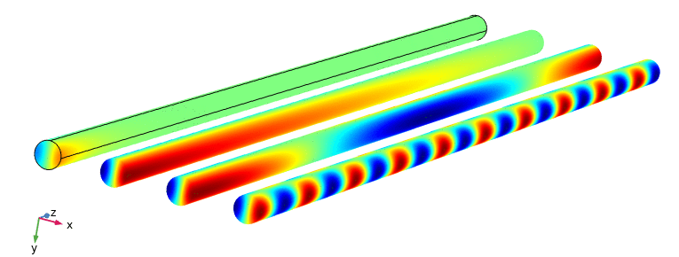
Starting from the left, the mode is excited below its cut-on frequency, so the axial wavenumber is imaginary and fairly large so the axial wavelength is fairly small, i.e. it cannot extend long into the tube. For the second tube, we are almost at the cut-on frequency of the mode, and so the axial wavenumber is very small, and so the wavelength is very long; in fact right at the cut-on frequency the mode in principle extends infinitely long, having an infinite phase speed, where only a transverse standing wave is seen, i.e. there is only variation in the cross-sectional direction. For the third frequency we are slightly above the cut-on, so the axial wvenumber is real, but the axial wavelength is still quite long. Only for the fourth frequency is it more clear to see that we have wave propagation. The difference between the lowest and the highest frequency in the above animation is only 10 %, so the modal behavior is highly dependent on the excitation frequency.
One important take-away from the above discussion is that you cannot in general simply measure the distance between two pressure peaks or dips in an acoustic field in a tube and deduce the excitation frequency, unless you know that you are dealing with a plane wave (as this exclusively has an axial wavenumber), or if a single mode carrying the sound field is excited well above its cut-on frequency.
So we are ready to clean up a couple of misconceptions, that I have heard or have had myself. A mode does not suddenly 'appear' out of the blue, just because the excitation frequency is above the cut-on frequency for the mode. Somewhere the tube is excited with a certain frequency and cross-sectional field characteristics and one or more modes will be excited depending on their cross-sectional characteristics and cut-on frequencies. Depending on the excitation frequency, some or none may appear only as evanescent waves, whereas as some or none will propagate. Why is 'none' included for propagation, didn't we say that the plane wave will always propagate? Yes, but only if it is excited in the first place! So if you excite a higher order mode, then only that mode will be seen in the tube, and whether it propagates or decays as an evanescent wave will depend on the excitation frequency. But if you don't have any kinks, bends, or other imperfections in your tube, only the mode(s) you excite will appear in the sound field. Input a plane wave and this will propagate on its own at an any frequency, without converting into other modes. The total sound field in a tube can always be described as a linear combination of the available modes, but this does not mean that going up in frequency results in e.g. a plane wave being converted into another mode.
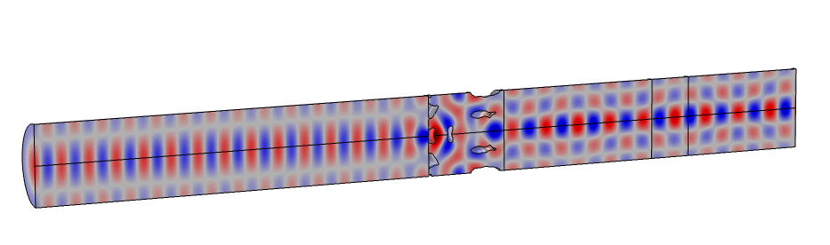
Speaking of mode conversion, with the above knowledge you should be prepared to appreciate how you can use optimization to manipulate modes, so that evanescent or propagation modes can converted into other modes, be they propagation or decaying. This is illustrated below for a (0,1)-to-(0,2) mode conversion, both propagating;
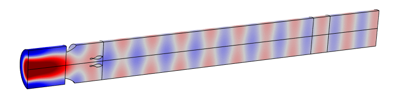
and for an evanescent (0,1)-to-(0,0) conversion, with the plane wave of course propagating;
Coming up with the idea for the above examples requires the knowledge of wave propagation in tubes in general, and so constantly studying the fundamentals is actually a great way to be innovative. A lot of engineers tell me that they would rather look into mathematics and physics when they need to, but if you don't have it in your toolboxes, you will never know that you could actually have needed the knowledge for an engineering problem in the first place. It is like keeping in shape, but for your mind; always sharpening the sword.
When it comes to experimental setup, must acoustic facilities only have a plane wave tube. This is understandable, but it would be really nice that students could study more complex sound fields via measurements. At least you can do simulations to get the insight, and I highly recommend COMSOL Multiphysics, as it has several useful features such a Ports, Eigenstudies, Boundary Mode studies, and more.
I hope you have gotten something out of this posts, and any comments or questions are appreciated.
Comments