#005: Transmission lines are awesome!
- Aug 1, 2017
- 2 min read
Updated: Jan 13, 2021
If you study engineering, you are likely to encounter the topic of transmission line model in a course like “Radio Frequency Fundamentals” or something to that effect. However, the concept of transmission lines is certainly not limited to electromagnetic propagation; for example, it has great usage within acoustics, as will be demonstrated now.
Imagine a straight tube carrying a propagating sound pressure:

The sound pressure is assumed constant in the cross-section, so that we have so-called plane wave propagation. The task is now to describe the sound field along the propagation axis. Since we can have several wavelengths along the tube, we need a so-called transmission matrix, which relates the four quantities 1) input pressure, 2) input volume velocity, 3) output pressure, and 4) output volume to each other. In its general form, this matrix system can be written as

The matrix elements are worked out [1] for a tube with length l and cross-sectional area S

with

So if the density and the sound speed are known, the tube is fully described. Other pairs of quantities that fully describe the tube are equally valid, but this will be touched further upon in upcoming blog posts. The wavenumber k is simply related to the sound speed.
In general, the density and the sound speed can both be complex. This way, so-called viscous and thermal losses can also be included in the transmission matrix for microacoustic applications. If you work with transmission line models in e.g. MATLAB, complex systems can be calculated efficiently, by combining cascaded and parallel systems. For Finite Element Modelling such systems can also be included, which can be very useful: Two larger volumes are connected via a tube with a circular cylindrical cross-section. The tube is not explicitly drawn or meshes; it is included as a mathematical abstraction using the excellent coupling and constraint options in COMSOL Multiphysics®[2].
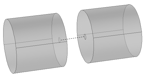
The dashed line indicates a mathematical description of a transmission line model for a circular cylindrical tube. Its cross-sectional area is indicated as interface surfaces on the two larger geometries.
The sound pressure level at one end of this system is found for a given velocity input at the other end, with the assumption that the tube is lossfree.

This sound pressure level matches the level that would have been found for a model with the tube included explicitly, but by including the tube only via mathematics you save degrees of freedom (thereby lowering solution time), especially for long tubes with thermoviscous losses included in the transmission matrix. It is also easier to run a parameter study on the length of the tube, since no geometry movement or remeshing is needed.
This brief introduction to transmission line modelling hopefully illustrates the power of this technique, and I would suggest employing it whenever possible. In future blog posts other related techniques will be described, which can also make calculations run more efficiently, and provide more insight than purely numerical models.
1): Propagation Of Sound Waves In Ducts, Finn Jacobsen, Acoustic Technology, Department of Electrical Engineering, Technical University of Denmark, Building 352, Ørsteds Plads, DK-2800 Lyngby, Denmark
2): COMSOL Multiphysics® v. 5.2. www.comsol.com. COMSOL AB, Stockholm, Sweden
Comments