#011: Reviewing BEM in COMSOL Multiphysics
- Dec 20, 2017
- 7 min read
Updated: Jan 13, 2021
COMSOL has just announced their newest 5.3a version with the acoustic boundary element method (BEM) implemented, much to many an engineer's delight. And this is truly very good news for those of us who work in the field of acoustics. I have earlier looked at, and tested, the prerelease version, and reported my findings to COMSOL, and in the following blog post the same tests have been carried out again using the final release. I hope you will get a better understanding of the method and the implementation.
Introduction:
The boundary element method solves the Helmholtz-Kirchhoff integral equation [1] numerically:
The equation states that the sound pressure in an arbitrary point can be found if you know both the pressure and the normal velocity in all points on a closed surface. That means that starting out you have infinitely many unknowns. For scattering problems, an incoming field can also be included in the calculations. Now you mesh the surface with a mesh with N nodes, and you have reduced your problem to 2N unknowns. Next, you assume that you know either the pressure or the velocity (or impedance) in all nodes. Now you have N unknowns. And finally, you create N equations by moving the observation point to each mesh node, one at a time. You then have to solve these equations numerically, with knowledge of the Green' functions for the particular problem and dimension. The great advantage is that you only have to mesh, and do calculations, for a surface, no matter where in the domain you want to extract your pressure. The downside is that the matrices will be fully populated, and so banding techniques or similar for sparse FEM matrices cannot be used, making the calculations more demanding.
One, perhaps trivial, comment on BEM in COMSOL: When you choose the dimension of the physics, choose the one you would have chosen using FEM instead, i.e. do not think about the mesh being one dimension lower in BEM than in FEM; just think about the physics in question, and let that determine the dimension.
Examples:
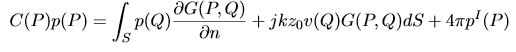
Scattering example 1:
Sphere being hit by plane wave, investigate total field, BEM vs FEM, ka=1.
There is a perfect match between BEM and FEM, not just for this frequency, but for all frequencies.

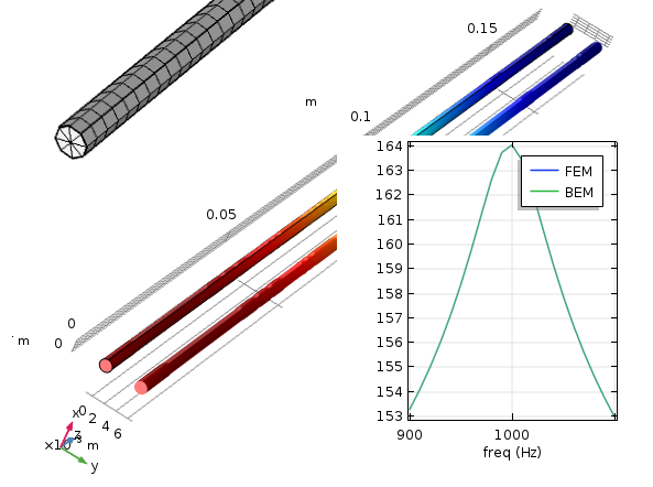
Scattering example 2:
One small oscillating sphere with one adjacent large rigid sphere, BEM only, to illustrate how an infinite void can have more than one mesh associated with it.
Tests:
A series of tests have been carried out to investigate some of the potential issues there can be with the boundary element formulation in general.
Complex media:
There is nothing in the boundary element formulation which should prevent having e.g. complex sound speed, as long as it is homogenous in the domain. Here, this has been tested by comparing BEM and FEM using a tube with a complex medium. There is a good match, and so it is actually possible to use complex media in the current BEM implementation.

Tri vs quad elements:
For the case used above, I also tried using a sweept mesh, so that the majority of elements are quad. This gives results similar to the above case with all tri elements.
Non-uniqueness:
For an exterior problem, interior resonances may pollute the exterior sound field. See [1] for details. This issue will be investigated via a test case: Sphere being hit by plane wave, investigate total field, BEM vs FEM, ka=3.14.
There is a perfect match between BEM and FEM, which would not be the case at this particular frequency, if COMSOL had not taken care of the non-uniqueness issue.
Thin body breakdown:
If two elements are placed very close together, e.g. one almost on top of the other, the numerical integration becomes an issue. There are remedies for this, see e.g. [2]. As I started looking into this issue, I realized there is no axisymmetric BEM formulation implemented. As I did not want to carry out this test with a 3D problem, I just looked at how the integration order can be set arbitrarily high (look under Quadrature), which should help, if the thin body issue should ever be a problem for you. It does not seem as if any special measures have been taken (yet) by COMSOL, but I may be wrong. Professor Vicente Cutanda (www.openbem.dk) can be contacted for more on this topic.
Discontinuous normals:
In isentropic acoustics, only normal velocities are considered. If a mesh node is shared by elements having significantly element normal, there can be a ambiguous interpretation of the velocity, see e.g. [3]. I used some simple test cases to try it out, and did not see any problems. In COMSOL MP you apply boundary conditions on boundaries, not nodes, so I think that this implementation takes care of this automatically. So no problems here.
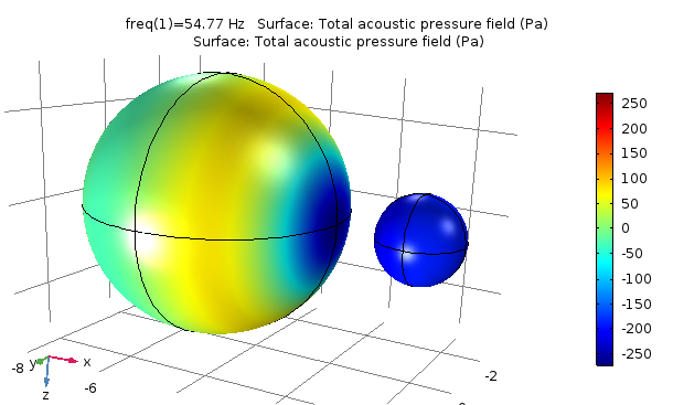
Low frequency breakdown:
Now it becomes interesting :-) As far as I can tell, this topic has been debated for some time, with no clear consensues(?) among the experts, so why not just test it out. The boundary element method in its standard should break down at low frequencies for interior problems, see [4] and [5] for details. I have never seen any issues for the practical applications I have calculated in the past using BEM in another software package, but I have also never investigated it. So let us have a look at it with an example:
A loudspeaker-like box has hard walls with one boundary having a constant displacement at all frequencies.
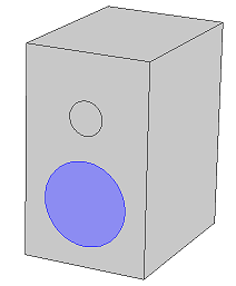
The air in the box should act like a spring, and so we would expect a constant pressure in the box at all low frequencies. Here is what I get:

We see that below 1 Hz, BEM cannot actually uphold a constant pressure in this particular box; instead of the displaced boundary seeing a constant compliance, the box simply exhibits the behavior of a pressure release. Okay, but would you ever run a loudspeaker simulation below 1 Hz? No! However, look here what happens if you drive a piston at one end of a tube in the millimeter range (when it comes to cross-section, not necessarily length), and look at the input impedance seen from the piston:

Now we actually see the problem below a higher frequency, approximately 200 Hz. The biggest potential problem with this is that so few people know the inner workings of BEM, and if they run such a simulation from 100 Hz and upwards, they can easily get confused about where the problem actually lies, since all resonances are picked up nicely with both FEM and BEM. Even the COMSOL support could potentially have trouble with this one: Imagine this as a support case for a simulation running from 100-10,000 Hz. The response seems fine, the resonances are properly placed (thermovisous losses have been omitted), but from 100 to 200 Hz the response is just off when compared to mesurements/analytical solutions/FEM. Imagine the detective work it would take to figure out this support case...
COMSOL is not at fault here; the issue is fundamentally related to the method, at least as I understand it. Although some remedies have been suggested, it could potentially clutter up the code. For most applications, it is certainly a non-issue, especially since you are probably better off using FEM for interior problems anyway, so there is absolutely nothing to be alarmed about. However, if you work with thermovisous acoustics and BEM (such as my friend Peter Risby Andersen, see [6] and https://www.researchgate.net/profile/Peter_Risby_Andersen), it becomes very important how the implementation acts in the extremes, e.g. small and narrow geometries. I am just trying shed light on any mathematical abnormalities, which could potentially lead to confusion (also see my motivation in blog post #001).
It would very nice if BEM experts such as Professor Peter Møller Juhl and Professor Vicente Cutanda could chime in on their observations in OpenBEM (www.openbem.dk) for similar applications, and perhaps Jörg Panzer with ABEC (http://www.randteam.de/ABEC3/Index.html), and Dr. Stephen Kirkup (http://www.boundary-element-method.com) would have some insight on the topic too. The low frequency breakdown was first brought to my attention about 10 years ago by Professor Dr. Sci. Sergey Sorokin ([5], http://personprofil.aau.dk/106335http://personprofil.aau.dk/106335), perhaps he could have some comments too? Let's get this thing closed once and for all :-)
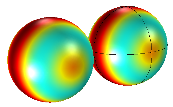
Finite void
I wanted to see if I could simulate a vibrating sphere inside a rigid sphere so that half of the mesh would look like this

and the rest of the mesh would just be the mirror image. I did not see any problems with this, so you can in general do interior problems with multiple meshes.

Couplings:
BEM acoustics in COMSOL MP can be coupled to FEM acoustics, FEM structural mechanics (solid, shell, ...), and possibly other physics. However, I did not see the option of coupling FEM thermovisous acoustics to BEM acoustics, but I believe it should be possible, so perhaps this will be put in a future release. Perhaps Technical Product Manager, Acoustics Mads Jensen has a comment to this? I think COMSOL has a very nice loudspeaker application that demonstrates the different couplings, so I will refer to their examples for more on this.
General comments:
BEM in COMSOL MP is a giant step forward, especially when solving exterior problems. They have to be of a certain size before the time consumption is less than FEM with PML and far-field calculation, but it is difficult to to say where the crossover is. You will of course have to experiment with this yourself.
I imagine that some future requests from users will be stuff like transient BEM, but on my part, I am happy with what we have now, although I would welcome an axisymmetry formulation in the future, to supplement the 2D and 3D formulation.
Oh btw. it is worth noting that you can now do a Polar Plot using the BEM pressure DOFs.
Conclusion:
The addition of acoustic BEM is very useful feature, especially if you have a good understanding of when to use it. COMSOL just keeps pushing the boundaries of multiphysics simulations, and I will continue to follow them with great interest. Go COMSOL!
[1]: "The Boundary Element Method for Sound Field Calculations", P.M. Juhl, PhD Dissertation, Department of Acoustic Technology, Technical University of Denmark
[2]: "On the Modeling of Narrow Gaps using the Standard Boundary Element Method", V.C. Henríquez, P.M. Juhl and F. Jacobsen, The Journal of the Acoustical Society of America, 109(4):1296-1303, 2001
[3]: "Discontinuous Boundary Conditions in the Boundary Element Method", R. Christensen, Course Code: TF24, University of Southern Denmark, 2008
[4]: "Analysis and Optimization in Structural Acoustics", S.T. Christensen, PhD Dissertation, Institute of Mechanical Engineering Aalborg University, 1999
[5]: "Low-frequency breakdown of boundary element formulation for closed cavities in excitation conditions with a ‘breathing’-type component", S. Sorokin and S.T. Christensen, Internation Journal for Numerical Methods in Biomedical Engineering, 2000
[6]: "Numerical Acoustic Models Including Viscous and Thermal losses: Review of Existing and New Methods", P.R. Andersen, V.C. Henríquez, N. Aage and S. Marburg, Proceedings of DAGA 2017, 2017
Comments