In this post we will have a look at modes for zero-dimensional systems, and how to relate eigenvalue/eigenvector analysis to more standard analyses of such systems, and how resonance comes into play in the whole thing.
0D
Certain systems can be described as being zero-dimensional. When this is the case, we don't explicitly include any spatial dimensions in our analysis. For example, we are not interested in how voltage varies inside a resistor along its length. Instead, we simply treat the entire component as a point; it has a certain component value associated with it to describe some internal properties, but it can be entirely lumped into a single entity. We often refer to such system as lumped parameter systems (Note: As mentioned in this post, there can in fact be some spatial direction and shape implicitly included in the 0D component, but we will not get in detail with this for now).
Let's look at an example to build some intuition. In electronics classes resonant behavior is often taught using an RLC-circuit with a Resistor, an Inductor (L), and a capacitor (C) as shown in Figure 1.

This is a so-called 1 degree-of-freedom (DOF) system with two 2 reactive components, so an order of 2. This is equivalent to a mechanical mass-spring-damper system, with their common velocity being the DOF, or a Helmholtz resonator in acoustics, with a common volume velocity as the DOF.
First we analyse the circuit with the means usually taught in electrical engineering:
- Decide on the transfer function you are interested in. In this case I want to see the common current (the DOF) for a given input voltage, so current divided by input voltage.
- Write the time-domain equation that describes the system behavior
- Transform to Laplace domain
- Set up the fraction that describes the desired transfer function...
...cast in a form that fits with
where the last part is included, as will prove useful later. The transfer function basically tells us all we need to know about the system. To fully understand this you need to have a look in an electronics book, or go to this blog post for my take on it. Let's try plugging in some numbers. To make things simple I choose some very unrealistic values, but it is really the relationship between them that is important:
I choose L=2 H, C=0.5 F, and R is left open for now. This gives us, by comparing the latter two equations,
and for our series connection
So there is a certain characteristic (angular) frequency associated with this circuit, and a quality factor Q related to all three components, and linearly dependent on 1/R; the lower the R, the higher the Q. Finally, the third factor that is needed to fully describe the circuit is the pass-band amplification, which here amounts to
found by comparing equations. So to reiterate: We have three components in our circuit, and three descriptive parameters, that are all we need. We can plot the complex transfer function as a function of the complex frequency s. This will require two plots in a 2D (real and imaginary) space, so we instead plot the amplitude level of the transfer function, as demonstrated in my previous post, here shown for a chosen value of R of 2 Ω:
We get a Q value of 1, and we know that this will give us complex roots.

We can find the response as a function of (angular) frequency as well as pole and zero placement, simply by plotting the transfer function in complex space, and looking at it from different angles. We see e.g. that at the maximum response value is -6dB which is the passband amplification (1/R) in dB for R=2 Ω. Nice, but...
...where the heck are the eigenvalues and eigenvectors that we were discussing in the last post?? Are they even here?
Yes, they are, but since electronics is typically not taught in the framework of state-variable analysis, it is often never outlined that there is an inherent eigenvalue problem associated with a circuit as shown in this example, or if it is, it is mentioned, but with important details left out. We will now try instead to use the state variable approach outlined in the previous post:
First we write the system as two first order equations and set them up in a matrix framework based on the relevant state variables, and leaving out the input. We can set up a matrix system like below
This is our second-order system written as two first-order equations in matrix form. This is the particular form of
As in the previous post, we assume solutions in the form of
so that we can finally write
for our electrical circuit. We can find the eigenvalues by first taking the determinant of (A-λI) where is the above matrix and I is the identity matrix, and setting it to zero
and then... we are actually done. Why? Look at the result. We have already seen it earlier. In the denominator of the transfer function. Which means:
The poles are the eigenvalues.
This actually makes sense. The pole placement tells us about where to expect singular behavior in the complex s-plane. As the poles come closer to iω-axis, the less damped it is, and the more of the singular characteristics is seen in the 'measurable' world. Similarly, we saw in the earlier post on modes that the eigenvalues are linked to behavior for which the system has a 'self-sustainability' character to it, i.e. where 'resonant' behavior can be expected, when an input/excitation is applied. What about the eigenvectors? Well, I think this is best illustrated via a structural mechanics example, rather than an electronics example, and also we add an extra degree of freedom to better show the meaning of the eigenvectors:
Assume that we have a two-degree-of-freedom (2DOF) system as shown below. We have two masses (the rectangles) and three springs (the zig-zag's). The black bars symboles rigid walls that two of the springs are connected two. There are other ways to set up 2DOF systems with e.g. two springs, but we will not dwell on that for now. With this setup, we can track the displacements of the masses with our eyes when animating, and these displacements will show us how the eigenvalues and -vectors relate to the physics.

The x's are the displacements, the m's are masses, and k's are spring stiffnesses. For the 2DOF system here, we can set up the equations of motion as
and
It is common to set the outer springs both to a stiffness of k, and the inner to a stiffness of K, and both masses to m. We can then cast the above in a matrix form as
What we now have to realize is that the above is simply
and so the associated eigenvalue equation can be written as
since when A is applied twice, the eigenvalue simply falls out twice. The above can be written as
Solving will give us four different eigenvalues, namely
and
Finally, we come to the eigenvectors: By inserting the eigenvalues back into the matrix, we get for the first eigenvalue (pair)
Hence, the only displacements that will fit with this eigenvalue are
which is equivalent to an associated eigenvector of
The eigenvector tells us at the eigenfrequency the ratio of the two displacements: A (1,1) eigenvector simply means that both masses have the same displacement. The eigenfrequency for this particular mode is
The minus/plus is related to our describing our time-dependency with a complex exponential. The physical displacement, however, will be real, and so only one distinct frequency will be associated with one distinct mode. The first mode has been animated with the help of MATLAB, here for unity values on all masses and springs:
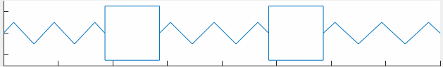
We see that the middle spring is decoupled, as it simply follows the movement of the masses, with no compression.
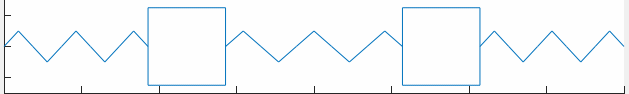
Similarly, for the other eigenvalue (pair) there is an associated eigenvector of
where the masses move exactly opposite of each other. with an associated eigenfrequency of
i.e. at a higher frequency than the first eigenmode. The displacement of the masses for this second mode is shown below
Remember, that we made some choices about the masses and springs; in general, these can have different values, and so this will affect both the eigenvalues and the eigenvectors. However, the analysis strategy will be the same as above.
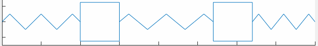
If the system is excited by an outside source, however briefly, it will have movement described by a superposition of the two eigenmodes, forever. This is because we haven't introduced any losses in the system. The reader should try and work out the equations, when one or more resistances are added, and see how it affects the eigenvalues and -vectors. Without losses, however, we can still learn a lot. We can for example examine so-called 'beating', where the middle spring is very compliant compared to the other two springs. If we then displace one of the masses, while keeping the other fixed, and let the mass go, we can see how in the beginning the movement will look like a 1DOF system, but the energy will start to be transferred to the other mass, and will slosh back and forth as shown below, where the second mass goes from moving to being still.
Now, there are many more topics that could be touched upon, such as forced responses, damping, orthogonality, 3-to-N DOFs, but for now we have at least seen how a system can have inherent modes, with associated frequencies and vectors, describing how the system will move on its own without a sustained force applied.
For more complex systems where it is not obvious how several DOFs are connected, and for high-order systems, the state-variable approach is useful for all the bookkeeping, and the user is encouraged to find usage of the state-variable approach for familiar problems that he or she is used to solving via other means. Also, remember as the order goes above 4 there are no algebraic solutions, and so we have to have other methods in the arsenal. However, as engineers we might not think about this, as we have software (e.g. electronics or mathematics software) in which everything is handled behind the scenes. Maybe that is part of the reason that you often don't have to be too concerned about eigenvectors in particular. Additional, for SISO systems we are often capable of lumping several components together as we know how series and parallel connections are handled in the s-domain, without having to be concerned with what happened to the original system branches and possible outputs that were not of interest to us. Therefore, we can lose touch of the matrix approach with its eigenvalues and eigenvectors, as we are mainly interested in one output DOF (current or voltage). You could argue that if you always work with transfer functions that are not too complex, you don't have to know about these details, but when you then have to work with more 'physical' engineering (structural mechanics, acoustics,...), you might have a harder time understanding certain concepts, and communication with other departments might be impaired.
As the eigenmodes can be used for describing system behavior, certain formulations exist that instead using the physical coordinates x1 and x2, instead use so-called normal coordinates related to each mode. In our case the normal coordinates would be x1+x2 and x1-x2, respectively. With these coordinates we know exactly the associated frequencies, that we have already calculated, with which the masses will oscillate. For a multiple degrees of freedom system, formulating the system via these normal coordinates can make our analysis simpler, but we will not get into this in the present blog post.
I hope the reader has gotten a little more knowledge about eigenmodes, eigenfrequencies, and eigenvectors. In upcoming posts we will look at 1D, 2D and 3D modes.
Additional notes
"A symmetric matrix with real entries has orthogonal eigenvectors".
"If we allow our matrix to have complex eigenvalues/-vectors, then the matrix does not have to be symmetrical (but it will be "normal"), to have orthogonal eigenvectors".
"If a matrix with real entries has complex eigenvalues, they will always exist in complex conjugate pairs.":
(For us not to have real entries in A, would mean complex component values.)